8. Searching and Sorting

8.1. The Sorting Problem

Do you stream music online? Do you click on a folder on your desktop to find and organize your files? Have you ever used Microsoft Excel to keep information in a spreadsheet? If we think for a moment about these software programs, we might realize that they have some features in common. One we might notice is that they eventually allow a user to sort information. In a music streaming app, you might choose to order your songs by title or by artist to make certain songs easier to find. When you’re looking at a folder full of files, you might order your files by file name or by the date it was last modified. In Excel, we can sort a column of data, which has the effect of rearranging the rows into a different order.

Sorting is a very common thing that programs do, and it is an interesting problem that can be tackled in a lot of different ways. In this introductory book you’re reading right now, we will look at only one of those ways. In doing so, we’ll also get better at walking through a problem logically in order to write a program that solves a problem. The end result will be that we improve our natural problem solving abilities, too. If you continue learning about computer science through other courses and other books, you’ll encounter other ways to perform sorting, some of which have really interesting capabilities. Well, what are we waiting for?

8.2. Towards an Algorithm for Sorting

In this section, we will start developing an algorithm for sorting. An algorithm is a series of well defined steps for solving a problem that has an input, an output, and completes in a reasonable amount of time. (The meaning of “reasonable” in this context is discussed in greater detail in more advanced computer science texts.)

Suppose we have a list of numbers, defined as such.

numbers = [8, 4, 3, 9, 5]

If we were to sort this list into ascending order, it would look like this.

numbers = [3, 4, 5, 9, 8]

A thoughtful reader might ask what happens if we have duplicate numbers. In other words, what if numbers were defined like this?

numbers = [3, 2, 3, 1, 4]

Note that we have two 3’s in our list. The sorted version would look like this.

numbers = [1, 2, 3, 3, 4]

The two 3’s remain preserved in the sorted list. We certainly wouldn’t want to lose items, so this makes sense. We used the word ascending to describe how we sorted the numbers, but that’s not technically correct since the list does not “ascend” between the first and second 3. A more correct phrase would be to describe the sort as monotonically increasing. We should use that phrase from here forward because 1.) it’s technically correct, and 2.) it sounds cooler.

So, how do we sort these numbers? In other words, how do we change the positions of the numbers in the list without losing any of the numbers?

Often, the best way to solve a problem is to think of a very simple instance of that problem, and then invent a simple solution. If we can find the smallest number in the list, where in the list should it go? The smallest number should always come first in the list, right?

Suppose we have the following list.

numbers = [8, 4, 3, 9, 5]

3 is the smallest number, so 3 should move to position 0, the start of the list. However, if we’re going to move the 3 to position 0, we need to find a new home for the 8. So, we’ll put 8 where the 3 was.

# Before
numbers = [8, 4, 3, 9, 5]
# After
numbers = [3, 4, 8, 9, 5]

None of the other numbers are touched in moving the 3 and the 8. Exchanging positions for the 3 and the 8 is called swapping the numbers. In fact, you learned how to swap values in a list back in Chapter 5. Now would be a good time to go back and view Listing 5.4 and Figure 5.2 in Section 5.1 again.

Now that the smallest item has been moved into position 0, we can do the same thing with the next smallest item. Where should the next smallest item go? In other words, what position should hold the next smallest item? If you said position 1, you’re correct!

# Original list
numbers = [8, 4, 3, 9, 5]
# Moving the smallest to position 0 by swapping.
numbers = [3, 4, 8, 9, 5]
# Moving the next smallest to position 1 by swapping.
numbers = [3, 4, 8, 9, 5]

Oh dear! Nothing changed! Actually, nothing needed to change. The 4 was already at its desired position. The computer doesn’t need to notice this. We don’t need to check to see if they swap needs to happen. We can always perform the swap, because we can swap a number with itself with no unfortunate side effects.

We can continue this procedure to move each subsequent number to the correct position in the list. When we have one final item remaining, we know that number is the biggest the number, and it should simply remain at the end of the list.

In each step x, we swap the next smallest value to position x. We scan across from position x to the end of the list, looking for and keeping track of the position of the smallest. When we are done scanning, we perform the swap. We can see what this procedure looks like in Figure 8.1. We’ve underlined the eventual position of smallest item that we have selected and swapped. In fact, this sort is named selection sort because of how we select the smallest item in each step.

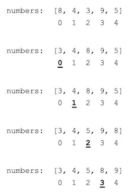
Fig. 8.1 Selection sort steps

There are a couple of things to note in the example shown that will help us write actual code. This is often how we come up with code that solves problems. We make up an example to help us think more concretely, and then we use that concrete example to help us see patterns that become our code. In Figure 8.1, you can see that we are starting each scan to find the smallest item at positions 0, 1, 2, and finally 3. 3 is one less than the last index in the list. We will need a loop to perform the scan to select the smallest item, and we will need another loop (outside of the scan loop) to control where we start each scan.

Try to write the code yourself before going on to the next section. Don’t cheat and look ahead. Make a focused attempt, hand-written on paper before you proceed.

8.3. The Selection Sort

Let’s walk through the advice given at the end of Section 8.2. Rather than name our list numbers, we’ll name it L (hey, fewer keystrokes!).

In each step of the selection sort, we scan across the list from beginning to end looking for the smallest item. We want to note the position/index where the smallest item sits (we’ll call it smallpos).

smallpos = 0
for i in range(1, len(L)):
    if L[i] < L[smallpos]:
        smallpos = i

This code assumes we start looking for the smallest at index 0. We let index 0 be the first smallest, and then we scan across from index 1 onward. However, we don’t want to start at index 0 every time. We want to start at index 0 to find the first smallest item, then we want to start at index 1 to find the next smallest, and so forth. So, the starting position needs to become a variable since the starting position needs to change each time. We’ll named that variable start. Notice how the code changes on lines 1 and 2 of the code.

smallpos = start
for i in range(start+1, len(L)):
    if L[i] < L[smallpos]:
        smallpos = i

Now that we have a start variable to control the starting position of each scan through the list, we need a loop to update it in each step of the algorithm.

for start in range(...):
    smallpos = start
    for i in range(start+1, len(L)):
        if L[i] < L[smallpos]:
            smallpos = i

What should we put in range in line 1? The first value of start should clearly be 0. What about the last value? From looking at Figure 8.1, we want the last time through the loop to be the next to last index. Therefore, the expression that ends the loop should be len(L)-1, like in the following code.

for start in range(0, len(L)-1):
    smallpos = start
    for i in range(start+1, len(L)):
        if L[i] < L[smallpos]:
            smallpos = i

This code now does successive scans across the list, but it doesn’t actually swap any values. Once we’re finished with the scan, but before we do another scan, we need to swap values between the positions stored in start and smallpos. The final solution is shown in Listing 8.1.

Listing 8.1 Selection Sort

for start in range(0, len(L)-1):
    # Find the smallest value and keep track of its position.
    smallpos = start
    for index in range(start+1, len(L)):
        if L[index] < L[smallpos]:
            smallpos = index

    # Swap the smallest value to the correct location,
    # i.e., where we started our walk through the list.
    temp = L[start]
    L[start] = L[smallpos]
    L[smallpos] = temp

This code works for any list we name L that has values that can be compared with the < operator. If we fill L with numbers, this code works. If we fill L with strings, it also works (can you guess how it orders strings?).

We can take this one step further and wrap it into a function that we can call. See Listing 8.2.

Listing 8.2 Selection Sort as a Function

def selsort(L):
    for start in range(0, len(L)-1):
        # Find the smallest value and keep track of its position.
        smallpos = start
        for index in range(start+1, len(L)):
            if L[index] < L[smallpos]:
                smallpos = index

        # Swap the smallest value to the correct location,
        # i.e., where we started our walk through the list.
        temp = L[start]
        L[start] = L[smallpos]
        L[smallpos] = temp

Then, we could call the function like this.

numbers = [3, 4, 1, 5, 2]
names = ["Becky", "Allen", "Derek", "Casey"]
selsort(numbers)
selsort(names)
print(numbers)  # Output is [1, 2, 3, 4, 5]
print(names)    # Output is ["Allen", "Becky", "Casey", "Derek"]

8.4. Searching for Items in Sorted Data

Human beings can find things easier in a list that has been sorted because they can eliminate sections of the list as they quickly visually scan its contents. Computers, too, can more easily find items in a list that has been pre-sorted.

Consider a long, unordered list of names. In order to determine if the name “Ned” exists in the list using a computer program, we would need to linearly scan the list from beginning to end. The number of comparisons we would need to do, in the worst case, would be equal to the number of items in the list.

Suppose, however, that the list is pre-sorted. We can reduce the number of comparisons between examining the middle item. If the name we seek comes before that middle item, we know that if the name exists in the list, it must exist in the first half of the list. Conversely, if the name we seek comes alphabetically after that middle item, we know that if the name exists in the list, it must exist in the latter half of the list. In that first step, we have eliminated half of all the items. This can speed up our search dramatically. Keep in mind that if the middle item is the name we were looking for in the first place, then we have found the name in only one comparison.

The algorithm we just described is called a binary search. To invent code that performs a binary search, let’s take the a similar approach to what we did with selection sort. We will start with an example, and observe patterns that we can turn into code.

Suppose we have a pre-sorted list L defined in the following way.

L = [2, 4, 7, 10, 13, 18, 25]

The middle item in this list happens to be 10, found at index 3. We know that 3 is the middle index because len(L) == 7 and 7 // 2 == 3 (recall that the // operator does integer division… it divides and then drops the fractional part).

Let’s try to find 18 in L. We compare 18 > 10 to find that 18 is greater than the middle. This means that if the 18 is in our list, it must be in the right half of the list. So, we now only need to look at the sublist [13, 18, 25]. We’ve reduced the number of items left to check to half!

So, how do we proceed from here? How do we keep track of which part of the list we’re currently examining. Well, as always, if we want to keep track of something or somethings, we use variables. Let’s let i and j be index variables that hold the positions of the leftmost item and rightmost item respectively. Let’s also create a variable m to calculate the index of the middle item. Figure 8.2 demonstrates the steps that will find 18 in L. Observe how i, j, and m change in each step.

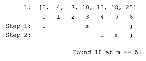
Fig. 8.2 Binary search steps, scenario 1

If 18 is greater than the middle (that is, if 18 > L[m]), then we move i to the right of m (that is, i = m + 1). What would be do if 18 were less than the middle? Then we would move j instead by moving it to the left of m (that is, j = m - 1).

We can see that in two steps, binary search is able to find the 18 in our example list. That’s fast! With a normal scan/search, it would have taken us 6 comparisons.

Wait a minute. What happens if we apply these same steps to look for a number that doesn’t exist in L. How about 17? Figure 8.3 walks us through that scenario.

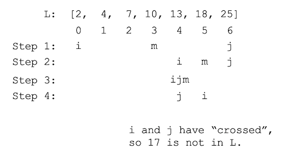
Fig. 8.3 Binary search steps, scenario 2

We are left with the idea that we will probably need to use a loop that continues to look for our target number, and the job of the loop’s body will be to either move i or j in each step. Terminal conditions for the loop are:

• We found our target number, or

• i and j have “crossed” (that is i > j), so our target number cannot be found

Okay, now its your turn. Can you attempt to construct the code for a binary search? Once the code is done, m should be set to the index of the found target number. If we don’t find the number, let’s set m to -1. Remember what we just said. We need a loop whose job (the body of the loop) is to move i and j and calculate m. The terminal conditions for the loop are given above. There may not be one single right way to write this code, so don’t worry about trying to do the one right way. Play around with it for a while on paper first. Try your best before looking ahead.

How far did you get? Where did you get stuck? You can learn a lot about how you solve problems and what types of things get you stuck by doing exercises like this.

Here is one possible solution.

x = 18   # x will be our target number
i = 0
j = len(L) - 1

while i <= j:
    # Find the middle index.
    m = (i + j) // 2
    if x < L[m]:
        # Look at the left half of L
        j = m - 1
    elif x > L[m]:
        # Look at the right half of L
        i = m + 1
    else:
        # Found it
        break

if i > j:
    m = -1

Note that x is not less than the middle and not greater than the middle, then it must be equal to the middle.

We can easily place this code into a function that we could call to find items in a list. We can pass to the function two values: 1.) the list L, and 2.) the target item x. The function should return the correct value of m, which should be -1 if we didn’t find the target item, or some integer >= 0 if we did find it. See Listing 8.3.

Listing 8.3 Binary Search as a Function

def binsearch(L, x):
    i = 0
    j = len(L) - 1

    while i <= j:
        # Find the middle index.
        m = (i + j) // 2
        if x < L[m]:
            # Look at the left half of L.
            j = m - 1
        elif x > L[m]:
            # Look at the right half of L.
            i = m + 1
        else:
            # Found it.
            return m

    # Didn't find x in the loop.
    return -1

8.5. (Optional) Using Recursion to Search

Binary search is a clever way to find a value in a list when the list values are in sorted order. Suppose we wanted to explain how it works to a friend. We might use the following description. If we want to find a value in an ordered list, look at the middle item. If that’s the value we want, great. We found it! If not, we ask if the value we want is smaller or larger than the middle. If its smaller, repeat the process again for the left “half” of the list. Otherwise, repeat it for the right “half” of the list.

Did you notice what we just did? We have recast the problem in terms of solving smaller versions of the problem itself. We could have said something like, “It the value isn’t in the middle, binary search either the left part or the right part.”

You might recall from Section 4.6 that this problem might be solvable using recursion. A recursive function is one that calls itself, though calling itself using a different parameter value each time.

The binary search function in the previous section was called with only two parameters, L and x. If you need to refresh your memory, take a look again at Listing 8.3. L was the list, and x was the value we wish to find. If we are going perform a binary search recursively, each time the binsearch function calls itself, it will need more information than just L and x. We will also need to pass the list indices that mark what part of the list that concerns us at that point. Let’s call the beginning index i and the end index j just like we did in the body of the function in Listing 8.3.

With this in mind, let’s define a new function named rbinsearch (the “r” makes us think of the word “recursion”) and let’s have the signature of that function become rbinsearch(L, x, i, j). Now, let’s use what we’ve learned about programming recursive functions. Often, we use an if statement. The first condition is the simplest. In this case, if i and j have crossed, we don’t have anything left in the list to search, so we can return -1. Otherwise, we can compute m as we did before. If x is at L[m], we found it and can return m. If not, we can recursively call rbinsearch. Try to write the code and define the function on your own. You can test your code using the following examples. If your function works properly, the code below should print True three times.

M = [1, 2, 7, 9, 13]
print(rbinsearch(M, 2, 0, len(M) - 1) == M.index(2))
print(rbinsearch(M, 13, 0, len(M) - 1) == M.index(13))
print(rbinsearch(M, 14, 0, len(M) - 1) == -1)

How did you do? Where did you get stuck? You can look at Listing 8.4 for an example solution. We should notice that calling rbinsearch is really clunky because we have to pass 0 and len(M) - 1 every time. We can redefine binsearch to call rbinsearch. In other words, binsearch(L, x) will call rbinsearch(L, x, 0, len(L) - 1). Sometimes programmers will call a function like rbinsearch a “helper” function, because the function you call in the first place (in this case, binsearch) then calls another function to do the actual work.

Listing 8.4 Recursive Binary Search

# The "helper" recursive function
def rbinsearch(L, x, i, j):
    if i > j:
        return -1
    else:
        m = (i + j) // 2
        if x == L[m]:
            return m
        elif x < L[m]:
            return rbinsearch(L, x, i, m - 1)
        else:
            return rbinsearch(L, x, m + 1, j)

# The function we actually call, which in turn calls the "helper" function.
def binsearch(L, x):
    return rbinsearch(L, x, 0, len(L) - 1)

8.6. Exercises

1. Demonstrate how selection sort would order the following list:

   [27, 34, 12, 9, 13]
   

   Show each step of the sort, even if that step does not move an item.

2. Demonstrate how selection sort would order the following list:

   ["carrots", "peas", "broccoli", "bok choy"]
   

   Show each step of the sort, even if that step does not move an item.

3. Suppose we have two lists that represent students’ names and their grade point averages (GPAs).

   names = ["Jennifer", "Alfred", "Jack"]
   gpas = [4.0, 3.1, 2.7]
   

   Also suppose that the names and GPAs line up with one another. In other words, Jennifer’s GPA is 4.0, Alfred’s GPA is 2.7, and Javier’s GPA is 3.1. If we were to sort names without also reordering gpas, Alfred’s GPA would become 4.0 (which I’m sure would make him happy, but it would be wrong).

   Define a function named sort_all that takes a list of lists. The function should sort the first list and then reorder all other lists in the same way as the first list.

   # Example 1:
   names = ["Jennifer", "Alfred", "Jack"]
   gpas = [4.0, 3.1, 2.7]
   sort_all([names, gpas])
   print(names)  # Output is ["Alfred", "Jack", "Jennifer"]
   print(gpas)   # Output is [3.1, 2.7, 4.0]
   
   # Example 2:
   names = ["Jennifer", "Alfred", "Jack"]
   gpas = [4.0, 3.1, 2.7]
   sort_all([gpas, names]) # we are sorting by GPA this time
   print(names)  # Output is ["Jack", "Alfred", "Jennifer"]
   print(gpas)   # Output is [2.7, 3.1, 4.0]